1 Overview
In the process of developing SDR products using the AD9361, in order to compress the spectrum of the digital baseband signal within a certain bandwidth, the shaping filter is obviously an indispensable component. This article gives the design process of the shaping filter, which is not only applicable to the AD9361 , also applicable to other wireless transceiver chips. Let’s first take a look at the spectrum of the rectangular pulse signal, as shown below
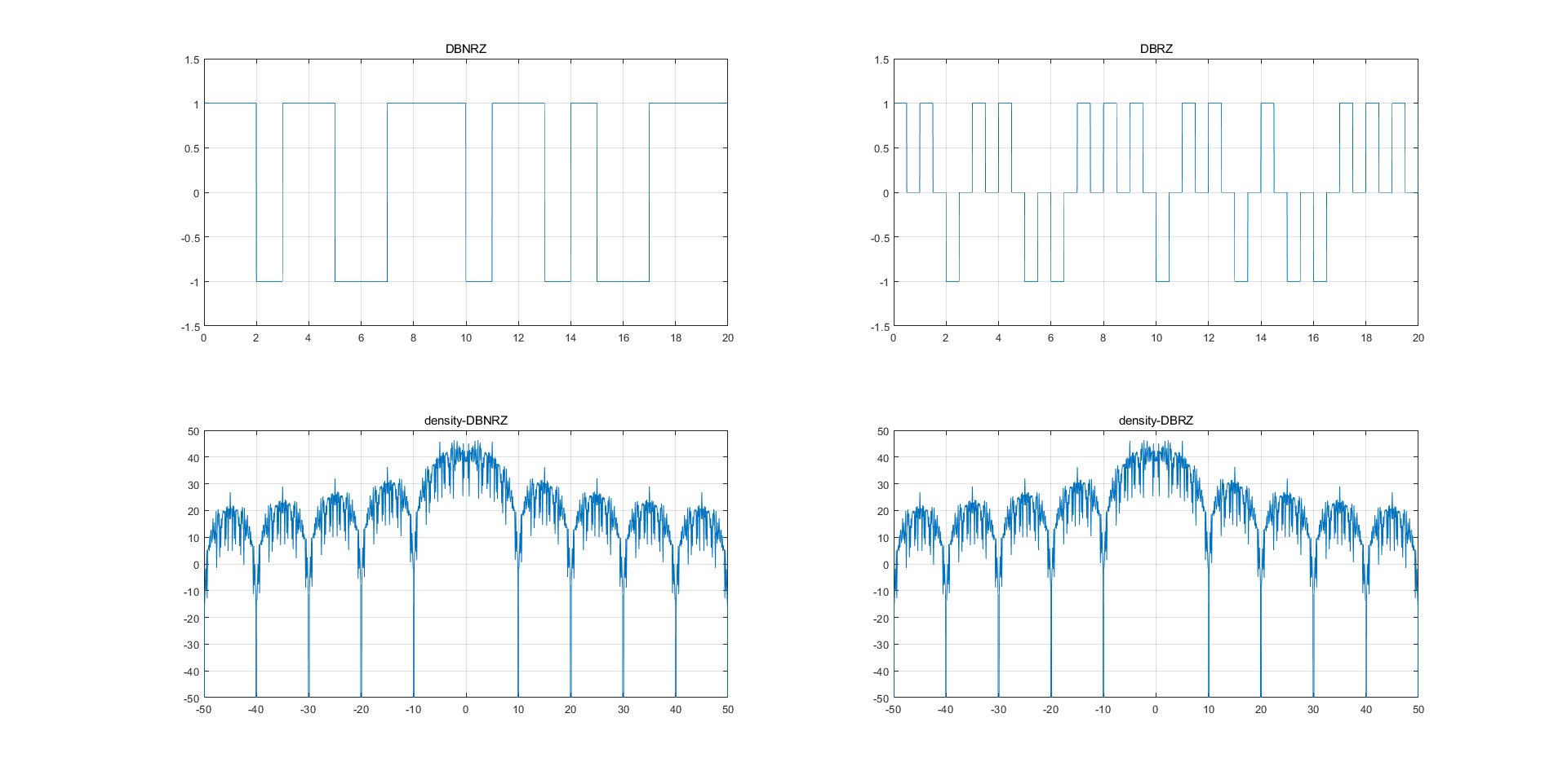
Obviously, if there are no restrictions on this spectrum, it will occupy a particularly large bandwidth. In actual wireless communication products, there are no products with this spectrum at all. Shaping filtering has two functions:
(1) Spectrum compression, limiting signal bandwidth. In digital communications, the baseband signal is a rectangular pulse. The sudden rising and falling edges contain rich high-frequency components, and their spectrum range is generally wide (the spectrum is a Sa function). In order to effectively utilize the channel, the signal needs to be spectrum compressed before signal transmission. This enables it to greatly improve frequency band utilization on the premise of eliminating inter-symbol crosstalk and achieving optimal detection. The signal bandwidth matches the channel bandwidth.
(2) Changing the shaped waveform of the transmission signal can reduce the impact of sampling timing pulse errors, that is, reducing inter-symbol interference (ISI). Signal band limitation will introduce inter-symbol crosstalk (discretization in the time domain corresponds to periodization in the frequency domain), which will cause distortion of the received signal waveform. But in general, it is only necessary that the signal sampling value at a specific moment is distortion-free, and it is not required that the entire signal waveform is distortion-free. The raised cosine filter can just band limit the baseband signal spectrum without affecting the signal at a specific moment.
2. Principle of shaped filter
Digital filters are divided into FIR (finite impulse response) and IIR (infinite impulse response). FIR has no feedback module, and IIR has a feedback module. As you can imagine, the output of FIR has nothing to do with the previous output, and the output of IIR is related to the previous output. One conclusion is: FIR has linear phase. Shaping filters generally use FIR filters. FIR filters have many structures, the simplest one is given in the figure below.
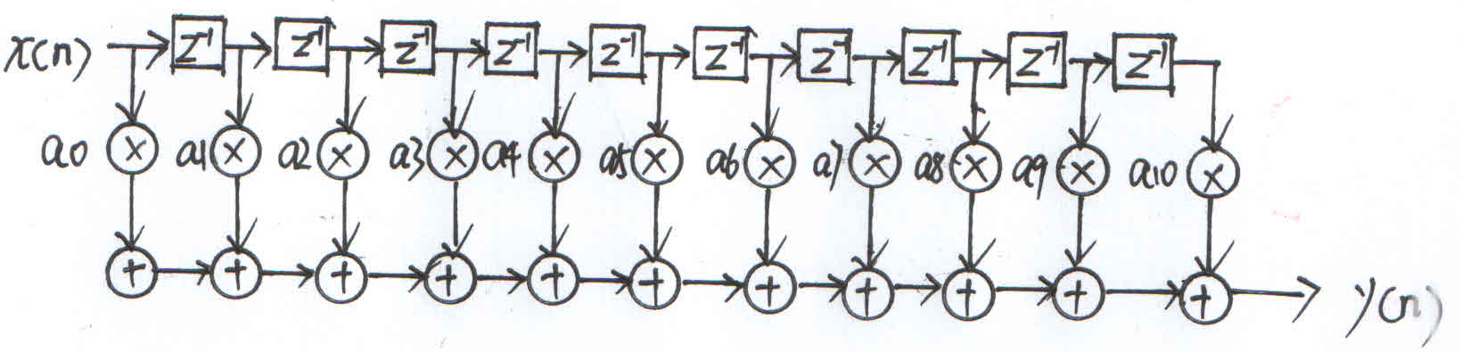
It can be seen that this is a structure of delay, multiplication and addition, which is actually a convolution sum, where x(n) is the input digital sequence, y(n) is the output digital sequence, a0-a10 is called the coefficient of the filter. The calculation process of convolution is: substitution, flipping, shifting, multiplication and summation. It is very vivid to scroll and sum at the same time. In order to verify this idea, we use Matlab to design a raised cosine filter, as shown below.
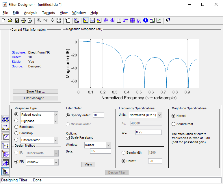
Quantize to 16 bits
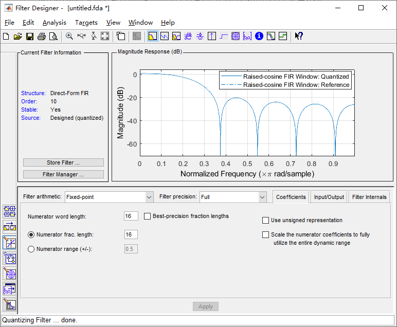
And save the quantized coefficients -2529,0,4654,10179,14661,16384,14661,10179, 4654,0,-2529
Assuming that the input sequence x(n) is [1,-1,-1,-1,-1,-1,-1,-1,1], the output of the filter can be calculated
y(0)=a0*x(0) =-2529
y(1)=a0*x(1)+a1*x(0)=2529
y(2)=a0*x(2)+a1*x(1)+a2*x(0)=7183
y(3)=a0*x(3)+a1*x(2)+a2*x(1)+a3*x(0)=8054
y(4)=……=2357
y(5)=……=-10581
Okay, this is the result of manual calculation. Let’s take a look at the output result of the Matlab function, as shown below.
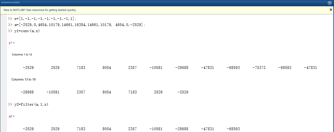
Among them, y1 is the result of the convolution operation, and y2 is the result of filtering using Matlab’s filter function. It can be seen that the first few output values of y2 and y1 are completely matched. The above process shows that the output of the digital filter is indeed the result of the convolution of the input sequence and the filter coefficients. There is another question, why do the spectral characteristics change after convolving the original digital sequence with the filter coefficients? A simple understanding is: the current output is the result of adding multiple previous input values multiplied by coefficients, which can smooth the input signal. Since the signal has become smoothed, signal mutations will not be so severe. , the frequency components of the signal must be reduced, and the spectrum is naturally compressed. Mathematically, the input and output of a digital filter can be expressed as a differential equation. The frequency response of this differential equation takes the form of low pass, high pass, band pass, etc., as stated in Oppenheim’s book “Signals and Systems” Very good explanation.
3. Implementation of shaping filter on FPGA
(1) First generate 20,000 random sequences of 1 -1 and save them in the rand_data.txt file. The Matlab code is as follows:
clear;clc;
N=20000;
s=randi([0 1],N,1);
s1=2*s-1;
fid=fopen('D:\Temp\matlab\rand_data.txt','w');
fprintf(fid,'%d\r\n',s1);fclose(fid);
(2) Generate a 128th-order square root raised cosine roll-off filter with a roll-off coefficient of 0.25 and a normalized cutoff frequency of 0.25, quantize it into a 16-bit integer, and save it in coe format for use by Vivado. The Matlab code is as follows:
clear;clc;
span=32; %span
sps=4; %samples per symbol
%use rcosdesign to get filter coefficients
h=rcosdesign(0.25, span, sps, 'sqrt');
%has to be divided by 2
h2=h/2;
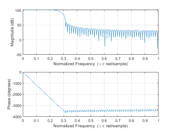
figure (1);
freqz(h2,1,1024);
%amplify and round coefficients
coe_int=round((h/max(abs(h)))*(2^15-1));
freqz(coe_int,1,1024);
format long;
%quantize coefficients to 15 decimal places
coe_frac=coe_int/2^15;
figure (2);
freqz(coe_frac,1,1024);
fid=fopen('D:\Temp\matlab\coe_frac.coe','w');
fprintf(fid,'Radix = 10;\r\n');
fprintf(fid,'CoefData =\r\n');
fprintf(fid,'%16.15f,\r\n',coe_frac);fprintf(fid,';');fclose(fid);
fid=fopen('D:\Temp\matlab\coe_int.coe','w');
fprintf(fid,'Radix = 10;\r\n');
fprintf(fid,'CoefData =\r\n');
fprintf(fid,'%d,\r\n',coe_int);fprintf(fid,';');fclose(fid);
fid=fopen('D:\Temp\matlab\coe_int.txt','w');
fprintf(fid,'%d ',coe_int);fclose(fid);The frequency response is as shown below
(3) Use the FIR IP core in Vivado, load the coe_int.coe file, and make the following configuration


(4) Write testbench, read the rand_data.txt generated in step (1), and save the FIR filtered results in filt_data.txt. Part of the code is as follows
integer fid_in;
initial
begin
fid_in = $fopen("D:/Temp/matlab/rand_data.txt","r");
end

always@(posedge clk_1m)
begin
if(!rst)
begin
din <= 8'd0;
s_data_tvalid <= 1'b0;
end
else if(s_data_tready)
begin
$fscanf(fid_in,"%d",din);
s_data_tvalid <= 1'b1;
end
end

integer fid_out;
initial
begin
fid_out = $fopen("D:/Temp/matlab/filt_data.txt","w");
end
always@(posedge clk_4m)
begin
if(m_data_tvalid)
begin
$fwrite(fid_out,"%d\n",dout);
end
end
(5) Configure Vivado to use Modelsim simulation and run it to get filt_data.txt.
(6) Check whether the results obtained by comparing filt_data.txt and Matlab using the filter function are consistent. The code is as follows
clear;clc;
ps=1*10^6; %symbole rate is 1MHz
Fs=4*10^6; %sample rate is 8MHz
N=2000; %lenth of simulation data
coe_int=importdata('D:\Temp\matlab\coe_int.txt');
s=importdata('D:\Temp\matlab\rand_data.txt');
fir_out=importdata('D:\Temp\matlab\filt_data.txt');
t=0:1/Fs:(N*Fs/ps-1)/Fs; %generate a time series of length N and frequency fs
%truncate the first 8K data of FIR output
fir_out_8k_temp=fir_out(2:N*(Fs/ps)+1,1);
fir_out_8k=fir_out_8k_temp';
%Sample at Fs frequency
ups=upsample(s',Fs/ps);
%filt
filt_mat=filter(coe_int,1,ups);
filt_mat_8k=filt_mat(1:8000);
%compare date
isequal(fir_out_8k,filt_mat_8k)
The comparison results are as follows

It can be seen that the output results of the FIR filter and the Matlab filter function are exactly the same.